Home > BrainVoyager > Data Preprocessing > Functional Preprocessing

Functional Preprocessing

Spatial Smoothing

1. Theoretical Background

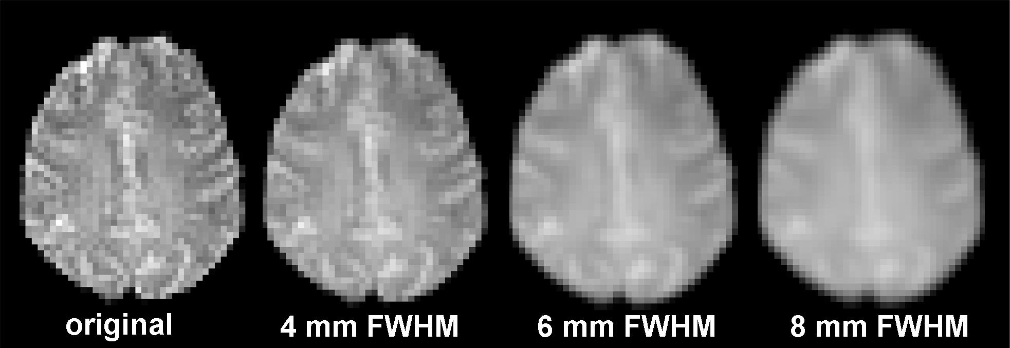
Spatial smoothing means that data points are averaged with their neighbours. This has the effect of a low pass filter meaning that high frequencies of the signal are removed from the data while preserving low frequencies. The result is that sharp "edges" of the images are blurred and spatial correlation within the data is more pronounced (see figure below).


EffectOfSmoothing

The approach of spatial smoothing is commonly used in fMRI studies and is justified by the fact that fMRI data inherently show spatial correlations due to functional similarities of adjacent brain regions and the blurring of the vascular system.

The standard procedure of spatial smoothing is employed by convolving the fMRI signal with a Gaussian function of a specific width.This so called Gaussian kernel is a kernel with the shape of a normal distribution curve. In the figure below you can see a standard Gaussian with a mean of 0 and a standard deviation of 1.

The size of the Gaussian kernel defines the "width" of the curve which determines in turn how much the data is smoothed. The width is not expressed in terms of the standard deviation σ, as customary in statistics, but with the Full Width at Half Maximum (FWHM). In this case the FWHM would be 2.35: The maximum of this curve is y = 0.4 at x = 0. The half maximum is y = 0.2 at x = -1.175 and at x = 1.175. Therefore, the full width of the curve at the point of the half maximum is about 2.35. Nevertheless, the FWHM is also related to the standard deviation σ as follows: FWHM = σ √(8 ln(2)).

There are several benefits associated with the application of spatial smoothing:

Improvement of the signal to noise ratio (SNR) => Increasing sensitivity
According to the matched filter theorem, the SNR reaches its maximum when the filter width matches the expected signal width. This, in turn, is of course dependent on the experimental design and the functional brain areas under investigation, e.g. Do you expect a narrow signal in the thalamus versus more extensive activations in the occipital lobe? Therefore, if a signal with a FWHM of 8 mm is expected the applied kernel size should be 8 mm as well.

Improving validity of the statistical tests by making the error distribution more normal
Most parametric tests assume normal error distributions and according to the central limit theorem the distribution of an average tends to be normal with a sufficiently large number of independent observations being averaged.

Accommodation of anatomical and functional variations between subjects
In multi-subject studies, individual brains are coregistered to each other to establish spatial correspondence between the different brains. Still, because of the substantial variation in individual brains, activated areas are rarely represented in exactly the same voxels. To increase the overlap of activated brain regions across subjects smoothing can be applied.

However, there are also some drawbacks which have to be carefully considered when specifying whether and to which extent spatially smoothing has to be applied:

Reduction of spatial resolution of the data
Spatial smoothing results always in reduced spatial resolution of the data. Therefore, it is important to decide whether a precise localization of the activations is important. However, even worse, if the filter width is set too small, there is practically no positive effect on the SNR while the spatial resolution is reduced.

Edge Artifacts
Along the edges of the brain, brain voxels are smoothed with non-brain voxels, resulting in a dark ring around the brain which might be mistaken for hypoactivity.

Merging
If activation peaks are less than twice the FWHM apart they are detected as a single activation rather than two separated ones.

Extinction
If the filter width is set too large, especially small meaningful activations might be attenuated below the significance threshold.

Mislocalization of activation peaks
As presented by Mikl and colleagues (2008), spatial smoothing almost unavoidably results in shifts of activation peaks. Therefore, as already mentioned above, it is crucial to decide what amount of spatial accuracy is required.

2. Spatial Smoothing in BrainVoyager

In general, spatial filtering is implemented in BrainVoyager by applying a 3D Gaussian kernel to the data. The width of the kernel can be either specified in mm or in pixels. Please note that the specification is only correct, if the "voxel resolution" has been indicated correctly. If you want to run Gaussian smoothing only within the slice plane, check the "2D" option instead of the default check mark in the "3D" option. This might be useful when the data set contains only few slices.  Furthermore, in the 2D space you can choose between smoothing in the "Space domain" or in the "Frequency domain". Both options show similar outcomes. However, for smoothing in the frequency domain, the image has to be first Fourier transformed, multiplied with the filter function and then back-transformed into the spatial domain which is accompanied by higher computational costs. Therefore, the space domain is checked by default. Nevertheless, for particularly large kernels (> 15 mm), smoothing in the frequency domain is recommended, since the computational cost of the spatial filter increases with the size of the filter kernel, whereas the costs for the frequency filter is independent of the filter width.

After BrainVoyager has finished spatial smoothing a new FMR is created whose file name is characterized by the options you used for filtering the data: "SD" for space domain versus "FD" for frequency domain, "3D" versus "2D", "SS" for spatial smoothing and the size of the filter kernel expressed in millimeter "mm" or pixels "px".

3. Comments on the Choice of the Kernel Size

Oversimplified, for single-subject analyses only modest filter sizes should be applied (about 4 mm), while for multi-subject analyses wider filters are reasonable to account for the intersubject-variability (about 6 -10 mm). However, to exploit the full spatial resolution of the data it is recommended to apply spatial smoothing only after having run single-subject analyses with no or only modest filter widths.

Furthermore, it is important to take into account that different preprocessing steps, like motion correction and creation of VTC files might also induce smoothing effects on the data depending on the interpolation method used. For example trilinear interpolation (often used because of its fast computation advantage) has the side-effect of “blurring” the data.
In sum, different factors have to be considered carefully, before deciding on the optimal kernel size.

In the figures below the effect of different smoothing kernels on the amount of significant activations is nicely visible (with the same statistical threshold):

No Smoothing

4 mm FWHM

6 mm FWHM

8 mm FWHM

Note: The AMR is detached in all four versions of this functional data set, otherwise you would not see the difference in the blurring factor!

References and Suggested Readings

  • Worsley KJ, Marrett S, Neelin P, Evans AC. Searching scale space for activation in PET images. Hum Brain Mapp 1996; 4: 74 - 90. (theoretical background)
  • Mikl M, Mareček R, Hluštik P, Pavlicová M, Drastich A, Chlebus P, Brázdil M, Krupa P. Effects of spatial smoothing on fMRI group inferences. Magn Reson Imaging 2008; 26: 490 - 503. (practical considerations)
Motion Correction

Head Motion in fMRI and Motion Correction in BrainVoyager

Head motion is probably the most severe but also an unavoidable problem in fMRI studies. Participants in fMRI studies are instructed not to move; however, it's impossible to lie completely still during a time interval of 1 to 2 hours. For well-trained experienced participants sub-millimeter movements can be achieved, but studies targeting children or patients are usually more affected by head motion problems, even after training participants before scanning.

This is a severe problem for statistical analysis of the data, since it is assumed that each voxel represents one unique location in the brain. If the subject however moved, the time course of one single voxel would represent a signal derived from different parts of the brain. In extreme cases, those effects might be visible in  “ring activations/deactivations” around the edges of the brain resulting from the fact that the intensity differences between adjacent voxels are particularly high at tissue boundaries.

To minimize those false-positive and false-negative activations while increasing sensitivity to true task-related activations, correction algorithms have to be employed to correct for motion artefacts.

In general motion correction incorporates the estimation of the movement based on one reference volume and the subsequent application of the estimated movement parameters to the data to realign the time series of brain images to the reference. The realignment is applied by rigid body transformations, which assume that the shape and size of the to be coregistered volumes are the same and that one image can be spatially matched to another one by the combination of three translation (in mm) and three rotation parameters (pitch, roll, yaw; in degrees). In the movies below, you can see for each parameter the respective movement direction and the plotting of the motion estimate.

Translation X:

Translation Y:

Translation Z:

Rotation X

Rotation Y

Rotation Z

Those motion estimates are visualized in a similar plot in BrainVoyager while motion correction is performed (see figure below).


By default BrainVoyager will also create a motion correction movie showing the difference between the first and last volume in the functional run before and after motion correction (upper and lower row). The last frame of this movie contains a difference image in which the first volume is subtracted from the last volume highlighting small differences in the intensities. Below you can see an example of a data set before and after motion correction. For more information, please consult the BrainVoyager User's Guide.

In addition to the plot and a motion-corrected data set (“_3DMCTS.fmr”), there are also two files saved to disk containing the motion estimates: “_3DMC.log” and “_3DMC.sdm”. While both files can be used to inspect the estimated motion parameters, only the sdm-file can be used to add the motion parameters as confounds to the general linear model since here these are saved in the format of a design matrix.

To save more detailed information about the motion estimates for each iteration step, check the “Create extended log file” option which results in an additional log file ending with “_3DMC_verbose.log”.

There are different options available in BrainVoyager allowing to adapt motion correction to the demands of the dataset. You can choose between three different interpolation methods: trilinear, sinc, or a combination of trilinear for detection of motion and sinc for correction. The method used is also indicated in the resulting filename following the _3DMC with T for trilinear, S for sinc and TS for a combination of both. While the computation cost of sinc interpolation is relatively high,  trilinear interpolation slightly smoothes the data spatially. Therefore, it is recommended to use the “Trilinear/sinc interpolation” option (default) to avoid the problem of inducing unwanted blurring effects in the data while preserving a reasonable computation time. Furthermore, only a subset of voxels can be used for the estimation of the movement parameters. In the standard application this is not necessary, but you can change this setting by (de)selecting the “Reduced data” option.

Even more parameters can be adapted in the “3D Motion Correction Options” dialog which can be evoked by clicking on the button “Options” in the “3D motion correction” field.
You can choose the reference volume for motion correction (default is the first volume) or even another reference FMR document for alignment. This reference dataset should have been acquired in the same scanning session as the current dataset. Choosing another FMR as reference for motion correction is often advantageous when another functional dataset was acquired closer in time to the anatomical data. This might improve the coregistration between function and anatomy, assuming there was not a lot of motion between the reference FMR and the current FMR. However, please note that this option is not meant for aligning different session FMRs, as it cannot easily correct big motion offsets.
By default the T1 saturated first volume fmr is also aligned to the reference volume. The reason for that is that it is often recommended to use the first volume fmr for the coregistration of the functional and anatomical data set, since the first volume is characterized by a more pronounced contrast which improves the alignment of the data.

There is also the possibility to correct for motion only in the x-y plane and to ignore the motion between slices by checking “Force 2D motion correction”. This is however only recommended, when the data set contains only very few slices (less than 5).
BrainVoyager masks out noise voxels by default using only voxels with an intensity above 100, when this value is set to 0 also voxels of the background are used for the motion correction process.
In the field “Parameter estimation for a volume” you can specify the maximum number of iterations used for each volume. This value is set to 100 which is very conservative and usually not necessary to estimate the motion parameters. Since head motion is usually incremental, meaning that motion increases from volume to volume over time, the parameter estimates of the last volume are used by default to start the estimation process of the motion parameters for the current volume. You can uncheck this option when you expect rather sudden movements to dominate the functional data set.

There are different motion patterns which have to be taken into account, as for example random motion, when the movement of the participant is unrelated to the experimental paradigm or task-correlated motion, which occurs for example in motor mapping experiments in which participants move in response to certain stimuli (e.g., button presses or overt speech). Not all kinds of motion can be corrected via the rigid body alignment. Slow motion drifts are usually well accounted for, but sudden motion spikes can pose a severe problem for the data quality even after preprocessing.
Motion-related artefacts can be addressed in a multitude of ways. A common addition to the rigid body alignment in the preprocessing pipeline is for example the inclusion of the realignment parameters (or an expanded set of these) as confounds in the general linear model, to mention only one of the discussed options in the literature to reduce residual motion effects on the data.

It is important to check the improvement of the data after motion correction. One tool that helps to evaluate the data quality and screen the functional time series for any problems is the “Time Course Movie” tool in the “Options” menu, which can display the volumes of the functional run over time. By running this tool you can check for any sudden intensity changes in the dataset or for movement across volumes. To easily detect motion, click the "First <--> Last " button, which alternate between the first and the last volume.
Note: It should be stressed that this tool is very useful to screen the data for any kinds of artefacts and data problems.

Below there are two time course movies switching between the first and last volume of the the same functional run. The first time course movie shows the data before motion correction, the second time course movie shows the data after motion correction.


There is no single accepted threshold for movement in functional runs, as the amount of "accepted" movement depends on many different factors, including the scanning parameters, the experimental design, the intended statistical data analysis and the movement pattern within a functional run.

Plotting motion using the created *_3DMC.sdm files in Matlab and Python

You can use the Maltlab or Python script attached to this article to create motion plots similar to the ones created by BrainVoyager.

The advantage is that you can load multiple *3DMC.sdm files at once. The output will be a *3DMC_MotionPlot.png file saved in the same folder as the *3DMC.sdm file. These scripts will also print for each run the maximum motion with respect to a reference run, the maximum motion within the same run, as well as the maximum range of motion within the same run. In case the reference run is the same as the current run, the maximum motion with respect to a reference run should be the same as the maximum motion within the same run.

Mean Intensity Adjustment
In the data of some scanners there might be global drifts over time, meaning tha... more
EPI artifacts and EPI distortion correction
Summary of EPI Artifacts Please find below a summary of echo planar imaging (EP... more
Including EPI distortion correction in Data Analysis Workflow
Since BrainVoyager 20, the creation of projects, pre-processing of projects, cor... more